1 Introduction

Time series forecasting is one of the most important fields in statistics because it is arguably the most impactful for businesses. Every business would love to know what will happen tomorrow, next week, next year, and next 10 years and make decisions accordingly. Although statistical methods for forecasting is not quite the silver bullet, it can help us make reasonable predictions under certain assumptions.

In this post, we will look into several forecasting models - both classical methods (e.g. ARIMA) and deep learing (LSTM, CNN) - and compare their performance using hyperparameter optimization with Optuna. I will also assume a business case in the end and the best model will be the less costly one. Let’s start with some data analysis and visualizations.

2 Data Analysis and Preprocessing

Firstly we will import the training dataset train.csv using pandas and check its columns and some sample values.

import pandas

local_filepath = "train.csv"
data = pandas.read_csv(local_filepath)
data.sample()

	row_id	date	country	store	product	num_sold
2025	2025	2017-02-12	France	KaggleMart	Kaggle Getting Started	291

data.describe()

	row_id	num_sold
count	70128.000000	70128.000000
mean	35063.500000	194.296986
std	20244.354176	126.893874
min	0.000000	19.000000
25%	17531.750000	95.000000
50%	35063.500000	148.000000
75%	52595.250000	283.000000
max	70127.000000	986.000000

# Check for missing values
True in data.isnull()

False

Good. The data don’t have any missing values. Now let’s check for what kind of values that the data have on each column.

print(f"Unique country values are: {data['country'].unique()}\n")
print(f"Unique store values are: {data['store'].unique()}\n")
print(f"Unique product values are: {data['product'].unique()}\n")
print(f"Unique dates are: {data['date'].unique()}\n")

Unique country values are: ['Belgium' 'France' 'Germany' 'Italy' 'Poland' 'Spain']

Unique store values are: ['KaggleMart' 'KaggleRama']

Unique product values are: ['Kaggle Advanced Techniques' 'Kaggle Getting Started'
 'Kaggle Recipe Book' 'Kaggle for Kids: One Smart Goose']

Unique dates are: ['2017-01-01' '2017-01-02' '2017-01-03' ... '2020-12-29' '2020-12-30'
 '2020-12-31']

So the table has the daily sales data of 4 different books, sold in 2 different stores, which have branches in 6 different countries, spanning from start of 2017 to the end of 2020. Data has 70128 rows which means for each book, store and country combination we have 4 years of sales data.

Let’s plot a subset of the whole data.

Code

import plotly.express as px

subsets = pandas.DataFrame()
subsets["subset1"] = data[
    (data["country"] == "Germany")
    & (data["store"] == "KaggleMart")
    & (data["product"] == "Kaggle Advanced Techniques")
].set_index("date")["num_sold"]

subsets["subset2"] = data[
    (data["country"] == "Belgium")
    & (data["store"] == "KaggleRama")
    & (data["product"] == "Kaggle Getting Started")
].set_index("date")["num_sold"]

subsets["subset3"] = data[
    (data["country"] == "France")
    & (data["store"] == "KaggleMart")
    & (data["product"] == "Kaggle Recipe Book")
].set_index("date")["num_sold"]

fig = px.line(
    subsets,
    width=700,
    height=500,
    title="Sales Data For Different Subsets",
    labels={"value": "Sales", "date": "Date", "variable": ""},
)
fig.show();

Looking at the plot, especially in the Subset1, there is a yearly seasonality in the sales. Also there is a sharp rise in the sales around New Year’s Eve.

Before modelling, we have to check whether any extra data transformation is needed. Since the data has 48 subsets like the 3 subsets above, it has to be arranged such that a subset’s all values for 4 years are in a sequence before continuing to another subset. Let’s create a sample DataFrame to illustrate this point.

import numpy as np

sample_countries = ["Germany", "France"]
sample_stores = ["KaggleRama", "KaggleMart"]
sample_timepoints = [0, 1, 2, 3]
sample_num_sold = np.tile([10, 20, 30, 40], 4)

idx = pandas.MultiIndex.from_product(
    [sample_countries, sample_stores, sample_timepoints]
)
example = pandas.DataFrame(index=idx, data={"num_sold": sample_num_sold})
example

			num_sold
Germany	KaggleRama	0	10
		1	20
		2	30
		3	40
	KaggleMart	0	10
		1	20
		2	30
		3	40
France	KaggleRama	0	10
		1	20
		2	30
		3	40
	KaggleMart	0	10
		1	20
		2	30
		3	40

Now transform the whole data.

from pandas import to_datetime

# First sort the data and drop the row_id column since we don't need it.
transformed_data = data.sort_values(by=["country", "store", "product", "date"]).drop(
    columns="row_id"
)

# Change the date column to pandas Datetime
transformed_data["date"] = to_datetime(transformed_data["date"])
transformed_data = transformed_data.set_index(["country", "store", "product", "date"])
transformed_data

				num_sold
country	store	product	date
Belgium	KaggleMart	Kaggle Advanced Techniques	2017-01-01	663
			2017-01-02	514
			2017-01-03	549
			2017-01-04	477
			2017-01-05	447
...	...	...	...	...
Spain	KaggleRama	Kaggle for Kids: One Smart Goose	2020-12-27	204
			2020-12-28	212
			2020-12-29	242
			2020-12-30	239
			2020-12-31	202

70128 rows × 1 columns

3 Modelling

The data is ready to model. We will create several different models for forecasting: ARIMA, Regression with ARIMAX and XGBoost, and Deep Learning with Long Short Term Memory (LSTM). Each model may need another data transformation but it will be easy to transform from the data that we have already preprocessed.

We will not tune the hyperparameters rigorously at first, just enough to get reasonable forecasts. After we went through all of them, I will create a custom performance metric for an assumed business case and then we will compare each model according to this metric.

3.1 STL-ARIMA

Autoregressive Integrated Moving Average (ARIMA) is a statistical method used for forecasting. It uses values at previous time points to predict current value (autoregression) and these regressions’ errors (moving average). Main assumption of ARIMA is that the time series should be stationary meaning its value is independent of time. Trend and seasonality makes the time series non-stationary. To make time series stationary we can use “differencing” - simply subtracting the value at t-1 from the value at t. “Integrated” part of the ARIMA is referring to the differencing order to make time series stationary.

ARIMA consists of three parts each having their own order - Autoregression p, Integration d, and Moving Average q. We will use Autocorrelation Function and Partial Autocorrelation Function graphs to select correct orders.

Moving to our data, just by looking the above plots we can say there is a strong seasonality in the time series but to quantify it we will use Kwiatkowski-Phillips-Schmidt-Shin (KPSS) test to check for stationarity.

from statsmodels.tsa.stattools import kpss

kpss_test = kpss(transformed_data)
print(f"p-value of KPSS test is: {kpss_test[1]}")

p-value of KPSS test is: 0.01

Null hypothesis of KPSS test is that the series is stationary. Since the p-value of our test result is smaller that 0.05 we can reject the null hypothesis and state that the series is non-stationary.

Before creating the ARIMA model we have to remove trend and seasonality from the data. We could use the seasonal variant of ARIMA called SARIMA; however, our data’s frequency is a day so it has a periodicity of 365 days. SARIMA models are more suitable for monthly or quarterly data; therefore we will use Seasonal-Trend Decomposition Using LOESS (STL) method to remove trend and seasonality from the data.

from statsmodels.tsa.seasonal import STL
import matplotlib.pyplot as plt
import pandas as pd
import seaborn as sns

# Setting plot style and size
sns.set_style("darkgrid")
plt.rc("figure", figsize=(7, 5))
plt.rc("font", size=10)

# Create a sample subset to plot
subset = transformed_data.loc["Germany", "KaggleRama", "Kaggle Advanced Techniques"]

# Plot the decomposed parts of the time series
stl = STL(subset, period=365, seasonal=7, trend_deg=1)
decomp = stl.fit()
fig = decomp.plot()
fig.show();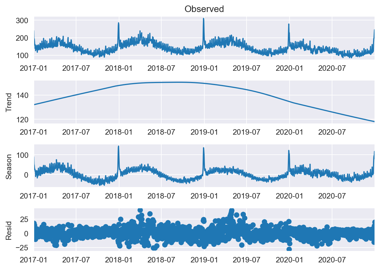

Above code decomposed the subset time series to three parts: trend, season, and residuals. Before creating ARIMA model, we still have to make sure that the residual part is non-stationary. We will test for stationarity with KPSS again and use differencing until it is stationary. This differencing degree will determine our I(d) parameter in the ARIMA model.

diff_test = kpss(decomp.resid)
print(f"p-value of KPSS test is: {diff_test[1]}")

p-value of KPSS test is: 0.1

Residual are stationary according to test so we won’t need a differencing in our model and therefore d degree will be 0. For the AR(p) order, we will look at the autocorrelation graphs. For the MA(q) order, we will try values and select the model with the lowest AIC (Akaike’s Information Criteria).

from statsmodels.graphics.tsaplots import plot_acf, plot_pacf

plot_acf(decomp.resid);
plot_pacf(decomp.resid);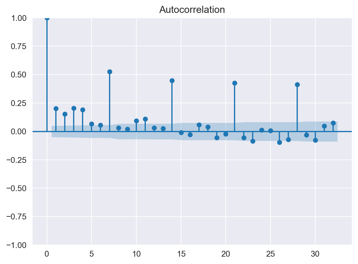

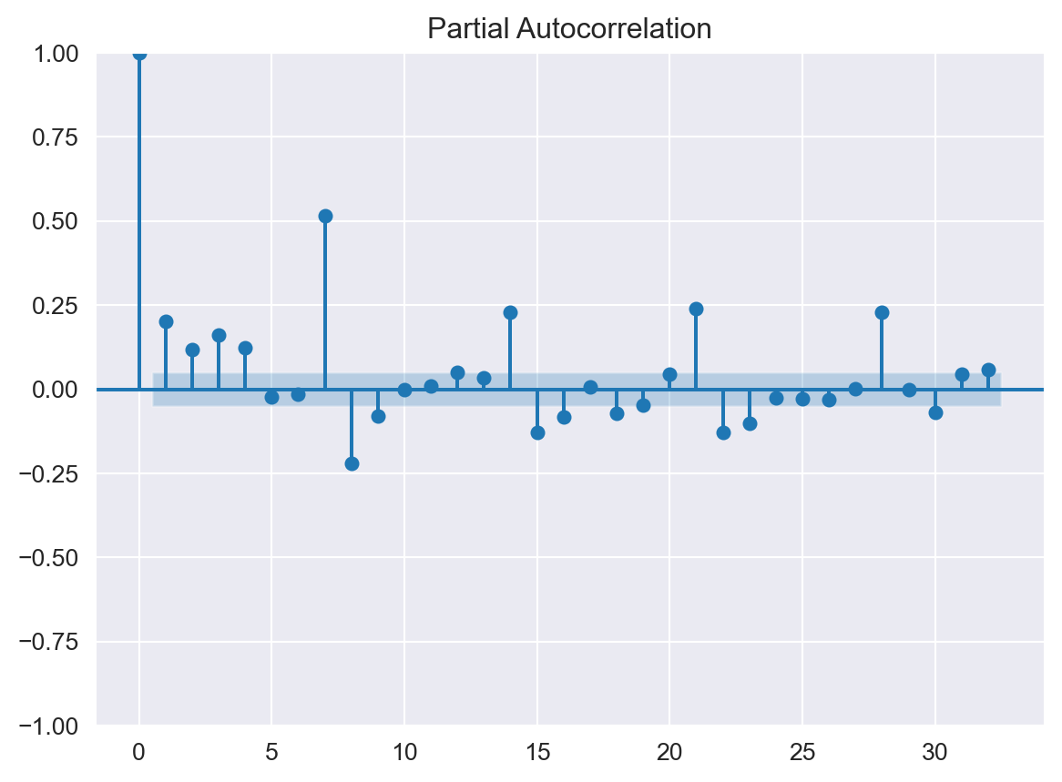
Partial Autocorrelation Function shows statistically significant correlations at lags up to 7; thus we will start with AR(7). Now it is a good time to split our subset to train and test parts. Train data will be the first three years’ data and the test will be last year’s data.

from statsmodels.tsa.forecasting.stl import STLForecast, STLForecastResults
from statsmodels.tsa.arima.model import ARIMA
from sktime.forecasting.model_selection import temporal_train_test_split

# Split subset to train-test
train_subset, test_subset_pretuning = temporal_train_test_split(subset, test_size=366)

# Define STLForecast model
stl_forecast = STLForecast(
    train_subset,
    model=ARIMA,
    model_kwargs={"order": (7, 0, 0), "trend": "t"},
    period=365,
    trend=1095,
    robust=False
)

# Fit the model
model = stl_forecast.fit()

# Forecast for the last year
forecast = model.forecast(steps=366)

# Create a function to plot both test data and forecast from the model to compare them visually.
def plot_forecasts(y_true, y_pred, title="Forecasts", width=700, height=500):
    # Create a DataFrame to store both series
    series = pandas.DataFrame()
    series["Observed"] = y_true
    series["Predicted"] = y_pred
    
    # Define plot attributes
    fig = px.line(
        series, 
        width=width, 
        height=height, 
        title=title,
        labels={
            "value": "Sales",
            "variable": ""
        }
    )
    fig.show()

plot_forecasts(test_subset_pretuning["num_sold"], forecast, title="STL-ARIMA Forecasts with (7,0,0)")
model.summary()

STL Decomposition and SARIMAX Results
Dep. Variable:	y	No. Observations:	1095
Model:	ARIMA(7, 0, 0)	Log Likelihood	-3477.975
Date:	Tue, 20 Dec 2022	AIC	6973.950
Time:	17:21:07	BIC	7018.937
Sample:	01-01-2017	HQIC	6990.973
	- 12-31-2019
Covariance Type:	opg

	coef	std err	z	P>\|z\|	[0.025	0.975]
x1	0.0074	0.135	0.055	0.956	-0.258	0.273
ar.L1	0.1083	0.019	5.696	0.000	0.071	0.146
ar.L2	0.1827	0.021	8.721	0.000	0.142	0.224
ar.L3	0.1113	0.018	6.122	0.000	0.076	0.147
ar.L4	0.1520	0.020	7.456	0.000	0.112	0.192
ar.L5	0.0204	0.020	1.024	0.306	-0.019	0.060
ar.L6	-0.0949	0.020	-4.857	0.000	-0.133	-0.057
ar.L7	0.5200	0.017	30.557	0.000	0.487	0.553
sigma2	33.3182	0.864	38.550	0.000	31.624	35.012

Ljung-Box (L1) (Q):	8.57	Jarque-Bera (JB):	629.83
Prob(Q):	0.00	Prob(JB):	0.00
Heteroskedasticity (H):	1.06	Skew:	-0.10
Prob(H) (two-sided):	0.60	Kurtosis:	6.71

STL Configuration
Period:	365	Trend Length:	1095
Seasonal:	7	Trend deg:	1
Seasonal deg:	1	Trend jump:	1
Seasonal jump:	1	Low pass:	367
Robust:	False	Low pass deg:	1

Warnings:
[1] Covariance matrix calculated using the outer product of gradients (complex-step).

The forecast looks pretty good already; however, from the summary we detect that p-value for Ljung-Box test is smaller than 0.05. The null hypothesis of Ljung-Box test is that residuals of the model after fitting ARIMA does not contain autocorrelations. Smaller than 0.05 p-value shows that our model could not capture the autocorrelations of the model fully. So will try different q orders and select the one which has the smallest AIC value and the case where the residuals are significantly autocorrelated (p > 0.05).

q_orders = np.arange(0, 8)
results = []
for q in q_orders:
    stl_forecast = STLForecast(
        train_subset,
        model=ARIMA,
        model_kwargs={"order": (7, 0, q), "trend": "t"},
        period=365,
        trend=1095,
        robust=False,
    )

    model = stl_forecast.fit()
    forecast = model.forecast(steps=366)
    results.append(model.model_result.aic)

print(f"Best q is {results.index(min(results))} with AIC value of {min(results)}")

Best q is 7 with AIC value of 6781.7431055363095

Let’s check the summary again with q value of 7.

stl_forecast = STLForecast(
    train_subset,
    model=ARIMA,
    model_kwargs={"order": (7, 0, 7),
                    "trend": "t"},
    period=365,
    trend=1095,
    robust=False
)

model = stl_forecast.fit()

# Forecast for the last year
forecast = model.forecast(steps=366)

# Plot both test data and forecast from the model to compare them visually.
plot_forecasts(test_subset_pretuning["num_sold"], forecast, title="STL-ARIMA Forecasts with (7,0,7)")

model.summary()

STL Decomposition and SARIMAX Results
Dep. Variable:	y	No. Observations:	1095
Model:	ARIMA(7, 0, 7)	Log Likelihood	-3374.872
Date:	Tue, 20 Dec 2022	AIC	6781.743
Time:	17:21:19	BIC	6861.719
Sample:	01-01-2017	HQIC	6812.005
	- 12-31-2019
Covariance Type:	opg

	coef	std err	z	P>\|z\|	[0.025	0.975]
x1	0.0307	0.042	0.725	0.468	-0.052	0.114
ar.L1	-0.5356	0.018	-29.124	0.000	-0.572	-0.500
ar.L2	-0.5941	0.025	-24.214	0.000	-0.642	-0.546
ar.L3	-0.2172	0.022	-9.847	0.000	-0.260	-0.174
ar.L4	0.3197	0.016	19.906	0.000	0.288	0.351
ar.L5	0.6246	0.022	28.755	0.000	0.582	0.667
ar.L6	0.4675	0.024	19.285	0.000	0.420	0.515
ar.L7	0.9349	0.018	52.310	0.000	0.900	0.970
ma.L1	0.8207	0.022	36.479	0.000	0.777	0.865
ma.L2	1.0375	0.034	30.775	0.000	0.971	1.104
ma.L3	0.7876	0.045	17.633	0.000	0.700	0.875
ma.L4	0.3276	0.046	7.110	0.000	0.237	0.418
ma.L5	-0.1245	0.040	-3.140	0.002	-0.202	-0.047
ma.L6	-0.1949	0.029	-6.761	0.000	-0.251	-0.138
ma.L7	-0.6672	0.021	-32.522	0.000	-0.707	-0.627
sigma2	27.4791	0.830	33.092	0.000	25.852	29.107

Ljung-Box (L1) (Q):	0.21	Jarque-Bera (JB):	359.53
Prob(Q):	0.65	Prob(JB):	0.00
Heteroskedasticity (H):	1.08	Skew:	0.07
Prob(H) (two-sided):	0.47	Kurtosis:	5.80

STL Configuration
Period:	365	Trend Length:	1095
Seasonal:	7	Trend deg:	1
Seasonal deg:	1	Trend jump:	1
Seasonal jump:	1	Low pass:	367
Robust:	False	Low pass deg:	1

Warnings:
[1] Covariance matrix calculated using the outer product of gradients (complex-step).

Finally calculate the mean absolute percentage error (MAPE) and R2 Score as a benchmark.

Code

from sklearn.metrics import mean_absolute_percentage_error, r2_score

print(f"MAPE for STL-ARIMA model is: {mean_absolute_percentage_error(test_subset_pretuning, forecast)}")
print(f"R2 Score for STL-ARIMA model is: {r2_score(test_subset_pretuning, forecast)}")

MAPE for STL-ARIMA model is: 0.18646794982275017
R2 Score for STL-ARIMA model is: -0.6091132358371121

3.2 Forecasting with Exogenous Regressors

Now we will move to the forecasting which uses exogenous variables as features. To achieve that, firstly, we will convert the datetime of the series to tabular features and then add holidays. We will also use some libraries dedicated to feature extraction from time series.

3.2.1 ARIMAX

For ARIMAX model, we will create a feature_matrix which has the date related features and lagged values as predictors.

import featuretools as ft
from sklearn.preprocessing import LabelEncoder, OneHotEncoder
import holidays
from statsmodels.tsa.deterministic import Fourier

# First we will create an EntitySet
entity_set = ft.EntitySet()
data = data.sort_values(by=["country", "store", "product", "date"])

# Specify index and time_index columns
entity_set.add_dataframe(
    dataframe_name="Datetime Features",
    dataframe=data,
    index="row_id",
    time_index="date",
)

feature_matrix, feature_defs = ft.dfs(
    entityset=entity_set,
    target_dataframe_name="Datetime Features",
    trans_primitives=["DAY", "MONTH", "WEEKDAY", "YEAR"],
)

# Label encode the year column
year_encoder = LabelEncoder()
feature_matrix["YEAR(date)"] = year_encoder.fit_transform(feature_matrix["YEAR(date)"])

# Get the holidays for each country
holidays_country = [holidays.country_holidays(i) for i in data["country"].unique()]

# Add the original date column for comparison
feature_matrix["date"] = to_datetime(data["date"])


"""
Check dates for local holidays. 
If there is a holiday on the date add their local name to holiday_name, else add "No Holiday".
"""
holiday_name = list()
for i in range(len(feature_matrix)):
    if feature_matrix["country"][i] == "Belgium":
        if feature_matrix["date"][i] in holidays_country[0]:
            holiday_name.append(holidays_country[0].get(feature_matrix["date"][i]))
        else:
            holiday_name.append("No Holiday")
    elif feature_matrix["country"][i] == "France":
        if feature_matrix["date"][i] in holidays_country[1]:
            holiday_name.append(holidays_country[1].get(feature_matrix["date"][i]))
        else:
            holiday_name.append("No Holiday")
    elif feature_matrix["country"][i] == "Germany":
        if feature_matrix["date"][i] in holidays_country[2]:
            holiday_name.append(holidays_country[2].get(feature_matrix["date"][i]))
        else:
            holiday_name.append("No Holiday")
    elif feature_matrix["country"][i] == "Italy":
        if feature_matrix["date"][i] in holidays_country[3]:
            holiday_name.append(holidays_country[3].get(feature_matrix["date"][i]))
        else:
            holiday_name.append("No Holiday")
    elif feature_matrix["country"][i] == "Poland":
        if feature_matrix["date"][i] in holidays_country[4]:
            holiday_name.append(holidays_country[4].get(feature_matrix["date"][i]))
        else:
            holiday_name.append("No Holiday")
    elif feature_matrix["country"][i] == "Spain":
        if feature_matrix["date"][i] in holidays_country[5]:
            holiday_name.append(holidays_country[5].get(feature_matrix["date"][i]))
        else:
            holiday_name.append("No Holiday")

feature_matrix["HolidayName"] = holiday_name

# Sort the dataframe so that date is sequential
feature_matrix = feature_matrix.sort_values(
    by=["country", "store", "product", "date"], ignore_index=True
)

"""
Check for the closeness of days to holidays. If a day is in the spectrum of 3 days before -
3 days after of a holiday, label it as Close.
"""
holiday_closeness = list()
for i in range(len(feature_matrix)):
    if feature_matrix["HolidayName"][i] != "No Holiday":
        holiday_closeness.append("Holiday")
    else:
        if len(list("No Holiday" == feature_matrix["HolidayName"][i - 3 : i + 4])) == 0:
            holiday_closeness.append("Close")
        elif False in list(
            "No Holiday" == feature_matrix["HolidayName"][i - 3 : i + 4]
        ):
            holiday_closeness.append("Close")
        else:
            holiday_closeness.append("Distant")
feature_matrix["HolidayCloseness"] = holiday_closeness

# One-hot encode holiday closeness
feature_matrix = pandas.get_dummies(
    feature_matrix,
    columns=[
        "country",
        "store",
        "product",
        "DAY(date)",
        "MONTH(date)",
        "WEEKDAY(date)",
        "YEAR(date)",
        "HolidayCloseness",
    ],
    drop_first=True,
)

# Deterministic Fourier Terms
## Yearly
yearly_fourier_terms = Fourier(365, 3)
index = np.arange(0, 1461)
yearly_fourier_terms = yearly_fourier_terms.in_sample(index)
cloning_func = lambda x: np.tile(x, 48)
yearly_fourier_terms = yearly_fourier_terms.apply(func=cloning_func, axis=0)
feature_matrix = feature_matrix.join(yearly_fourier_terms, how="left")

# Edit columns
feature_matrix = pandas.DataFrame.join(
    feature_matrix.drop(columns=["num_sold", "HolidayName"]),
    feature_matrix["num_sold"],
    how="left",
)

feature_matrix

	date	country_France	country_Germany	country_Italy	country_Poland	country_Spain	store_KaggleRama	product_Kaggle Getting Started	product_Kaggle Recipe Book	product_Kaggle for Kids: One Smart Goose	...	YEAR(date)_3	HolidayCloseness_Distant	HolidayCloseness_Holiday	sin(1,365)	cos(1,365)	sin(2,365)	cos(2,365)	sin(3,365)	cos(3,365)	num_sold
0	2017-01-01	0	0	0	0	0	0	0	0	0	...	0	0	1	0.000000e+00	1.000000	0.000000e+00	1.000000	0.000000e+00	1.000000	663
1	2017-01-02	0	0	0	0	0	0	0	0	0	...	0	0	0	1.721336e-02	0.999852	3.442161e-02	0.999407	5.161967e-02	0.998667	514
2	2017-01-03	0	0	0	0	0	0	0	0	0	...	0	0	0	3.442161e-02	0.999407	6.880243e-02	0.997630	1.031017e-01	0.994671	549
3	2017-01-04	0	0	0	0	0	0	0	0	0	...	0	0	0	5.161967e-02	0.998667	1.031017e-01	0.994671	1.543088e-01	0.988023	477
4	2017-01-05	0	0	0	0	0	0	0	0	0	...	0	1	0	6.880243e-02	0.997630	1.372788e-01	0.990532	2.051045e-01	0.978740	447
...	...	...	...	...	...	...	...	...	...	...	...	...	...	...	...	...	...	...	...	...	...
70123	2020-12-27	0	0	0	0	1	1	0	0	1	...	1	0	0	-6.880243e-02	0.997630	-1.372788e-01	0.990532	-2.051045e-01	0.978740	204
70124	2020-12-28	0	0	0	0	1	1	0	0	1	...	1	0	0	-5.161967e-02	0.998667	-1.031017e-01	0.994671	-1.543088e-01	0.988023	212
70125	2020-12-29	0	0	0	0	1	1	0	0	1	...	1	1	0	-3.442161e-02	0.999407	-6.880243e-02	0.997630	-1.031017e-01	0.994671	242
70126	2020-12-30	0	0	0	0	1	1	0	0	1	...	1	1	0	-1.721336e-02	0.999852	-3.442161e-02	0.999407	-5.161967e-02	0.998667	239
70127	2020-12-31	0	0	0	0	1	1	0	0	1	...	1	1	0	-9.797174e-16	1.000000	-1.959435e-15	1.000000	-2.939152e-15	1.000000	202

70128 rows × 69 columns

The feature matrix is almost ready for use in ARIMAX model. To summarize what we have done so far regarding the features, we have transformed the time points to categorical variables - day of the month, weekday, and year and added holidays. To better account for the effect of holidays, we have created three dummy holidays variables: Close, Distant and Holiday. Then to capture yearly seasonality we have added Fourier terms with period of 365. After creating the subset we can discard the country, product and store variables since we are training the models for each combination and they add nothing of value for forecasting in this case.

Let’s create the ARIMAX model and forecast with the same subset.

from statsmodels.tsa.arima.model import ARIMA
from statsmodels.tsa.statespace.sarimax import SARIMAX

# Create the same subset but this time with features.
subset_reg = feature_matrix[
    (feature_matrix["country_Germany"] == 1)
    & (feature_matrix["store_KaggleRama"] == 1)
    & (feature_matrix["product_Kaggle Recipe Book"] == 1)
]
subset_reg = subset_reg.drop(
    columns=[
        "date",
        "country_France",
        "country_Germany",
        "country_Poland",
        "country_Italy",
        "country_Spain",
        "store_KaggleRama",
        "product_Kaggle Getting Started",
        "product_Kaggle Recipe Book",
        "product_Kaggle for Kids: One Smart Goose",
    ]
)

# Train - Test Split
train_reg, test_reg = temporal_train_test_split(subset_reg, test_size=366)

# Define endogenous and exogenous variables
endog = train_reg["num_sold"]
exog = train_reg.drop(columns="num_sold")

# Use the same orders as previous ARIMA model
arimax_model = ARIMA(
    order=(3, 1, 3), endog=endog, trend=[0, 1], exog=exog, enforce_stationarity=True
)

arimax_results = arimax_model.fit()

# Forecast for the last year
forecast_reg = arimax_results.forecast(366, exog=test_reg.drop(columns="num_sold"))

test_reg = test_reg.set_index(forecast_reg.index)

# Plot both test data and forecast from the model to compare them visually.
plot_forecasts(test_reg["num_sold"], forecast_reg, title="ARIMAX Forecasts");

From the plot we can see that this model performs worse than STL-ARIMA model. Let’s check ARIMAX model’s MAPE score to quantify performance difference.

Code

print(f"MAPE for ARIMAX model is: {mean_absolute_percentage_error(test_reg['num_sold'], forecast_reg)}")
print(f"R2 Score for ARIMAX model is: {r2_score(test_reg['num_sold'], forecast_reg)}")

MAPE for ARIMAX model is: 0.6281181684643169
R2 Score for ARIMAX model is: -7.921475722370131

3.2.2 XGBoost

Let’s try the regression now with using XGBoost. We will again use the same feature matrix as exogenous variables but we’ll also use previous values of num_sold as input variables.

from sklearn.preprocessing import MinMaxScaler

# Create a function so that we can try with different window sizes
def prev_values_tabularizer(feature_matrix, endog, window_size, scaler=False):
    # Create a list to store previous values
    prev_values = list()
    for i in range(len(feature_matrix)):
        prev_values.append(feature_matrix[endog][i : i + window_size])

    # Reshape from columns to rows
    prev_values = [
        pandas.Series(prev_values[i]).values.reshape([1, -1])
        for i in range(len(prev_values))
    ]

    # Create placeholder DataFrame with zeros and change them with previous values
    zeros_matrix = np.zeros(shape=[len(feature_matrix), window_size])
    placeholder_df = pandas.DataFrame(zeros_matrix)
    for i in range(len(placeholder_df)):
        for j in range(window_size):
            try:
                placeholder_df[j][i] = prev_values[i][0][j]
            except IndexError:
                continue

    # Add previous values to feature matrix, shift it by window size, remove first window size values from the feature matrix
    feature_matrix = pandas.concat([feature_matrix, placeholder_df], axis=1)
    feature_matrix[list(range(window_size))] = feature_matrix[
        list(range(window_size))
    ].shift(window_size)
    feature_matrix = feature_matrix.drop(list(range(window_size)), axis=0)

    # If scaler is passed, apply scaling to previous values of endogenous variable
    if scaler != False:
        feature_matrix[list(range(window_size))] = scaler.fit_transform(
            feature_matrix[list(range(window_size))]
        )

    # Reorder the columns so that endogenous variables are at the far most right
    reordered_columns = (
        feature_matrix.columns.to_list()[: (-window_size - 1)]
        + feature_matrix.columns.to_list()[(-window_size):]
        + [feature_matrix.columns.to_list()[(-window_size - 1)]]
    )
    feature_matrix = feature_matrix[reordered_columns]

    return feature_matrix


scaler = MinMaxScaler()

# We use 7 as window_size because of the previous partial autocorrelation graphs
regression_matrix = prev_values_tabularizer(feature_matrix, "num_sold", 7)

We have transformed the feature matrix suitable for forecasting with regression. Now we have to split it again to train and test subsets and create regression model with XGBoost.

from xgboost import XGBRegressor

# Create the same subset as previous examples and split
subset_xgboost = regression_matrix[
    (regression_matrix["country_Germany"] == 1)
    & (regression_matrix["store_KaggleRama"] == 1)
    & (regression_matrix["product_Kaggle Recipe Book"] == 1)
]
subset_xgboost = subset_xgboost.drop(
    columns=[
        "date",
        "country_France",
        "country_Germany",
        "country_Poland",
        "country_Italy",
        "country_Spain",
        "store_KaggleRama",
        "product_Kaggle Getting Started",
        "product_Kaggle Recipe Book",
        "product_Kaggle for Kids: One Smart Goose",
    ]
)

train_subset_xgboost, test_subset_xgboost = temporal_train_test_split(
    subset_xgboost, test_size=366
)

# Define train/test features and targets
train_targets_xgboost = train_subset_xgboost["num_sold"]
train_features_xgboost = train_subset_xgboost.drop(columns="num_sold")
test_targets_xgboost = test_subset_xgboost["num_sold"]
test_features_xgboost = test_subset_xgboost.drop(columns="num_sold")

# Define model
xgboost_model = XGBRegressor()
xgboost_model.fit(train_features_xgboost, train_targets_xgboost)

# Forecast for the last year
forecast_xgboost = pandas.DataFrame(xgboost_model.predict(test_features_xgboost))
forecast_xgboost.set_index(test_features_xgboost.index, inplace=True)

# Plot both test data and forecast from the model to compare them visually.
plot_forecasts(test_targets_xgboost, forecast_xgboost, title="XGBoost Forecasts");

From the plot we can see that regression model with XGBoost performs better than ARIMAX model. Let’s check the scores again.

Code

print(f"MAPE for XGBoost Model is: {mean_absolute_percentage_error(test_targets_xgboost, forecast_xgboost)}")
print(f"R2 Score for XGBoost Model is: {r2_score(test_targets_xgboost, forecast_xgboost)}")

MAPE for XGBoost Model is: 0.09307335208975362
R2 Score for XGBoost Model is: 0.6931165642563528

Scores surely seems better than our other forecasting attempts with STL-ARIMA and ARIMAX, though it can be said that this regression model tends not to undershoot. It is also more successful to capture New Year’s Eve sales than other models.

It is still early to call this the best model, since we didn’t tuned thoroughly the models’ hyperparamaters and there are deep learning models to try. Now we’ll move to the business case definition and after that, hyperparameter tuning of STL-ARIMA, ARIMAX, and XGBoost models. For deep learning part of this case please refer to Part 2.

4 Business Case Objective Function

To compare different models, so far, we have used Mean Absolute Percentage Error and R2 Scores. We have also plotted our forecasts and compared them with test targets. Now we will approach the problem from a different perspective.

Instead of minimizing error, we will try to minimize our cost. It didn’t matter whether a sales forecast is for example 20 units more or less; but having 20 more books in the inventory and opportunity cost of selling 20 less books may not be the same. Our custom function will define exactly that.

Our assumptions are:

Every book is sold for €20
Book dimensions: 210x148x10mm (A5)
Storage cost: €100 per month
Warehouse dimensions: 2x2x3m
Warehouse space utilization: %15

With these assumptions, one warehouse can store approximately 6000 books for a storage fee of €100 per month. The scenario is that for every each book which the forecast undershoots the true sales, we have the opportunity cost of one book. If the forecast overshoots the true sales, then we can store the book in our warehouse by renting it. After renting the warehouse, each subsequent undershoot can be compensated from our inventory - effectively eliminating the opportunity cost but if storage limit is exceeded then we have to rent another warehouse increasing our monthly cost to €200.

We will use the function cost_function() to calculate this metric.

# Define cost function for our case
def cost_function(storage, y_true, y_pred, book_price, storage_monthly_rent):
  if storage == 0:
    if y_pred <= y_true:
      cost = book_price*(y_true - y_pred)
      to_storage = 0
      return cost, to_storage
    elif y_pred > y_true:
      cost = storage_monthly_rent/30
      to_storage = y_pred - y_true
      return cost, to_storage
  elif storage > 0:
    if y_pred <= y_true:
      if (y_true - y_pred) < storage:
        cost = storage_monthly_rent/30
        to_storage = y_pred - y_true
        return cost, to_storage
      elif (y_true - y_pred) > storage:
        cost = book_price*(y_true - y_pred - storage) + storage_monthly_rent/30
        to_storage = -storage
        return cost, to_storage
    elif y_pred > y_true:
      cost = storage_monthly_rent/30
      to_storage = y_pred - y_true
      return cost, to_storage

5 Hyperparameter Tuning with Optuna

Now we will tune and select hyperparameters for our models with the lowest cost. To reduce bias and get better generalization from the models, we will split the data to train - test - validation. While searching for the model with lowest cost using test data it may overfit. Therefore, we will tune the parameters using test dataset and after that check the performance using validation data.

Also earlier we were using test features for forecasts but feature matrix contains future num_sold values in it; thus, it wasn’t a legitimate forecast. In this part we will also change the way forecasts are created so that the model uses its own forecasts as past values instead of real sales.

5.1 STL-ARIMA Tuning

import optuna
import statsmodels

# Create validation data for STL-Arima
train_subset = subset["num_sold"][0:730].reset_index().drop(columns="index")
test_subset = subset["num_sold"][730:1095].reset_index().drop(columns="index")
val_subset = subset["num_sold"][1095:1461].reset_index().drop(columns="index")

# Define Optuna Objective
def stl_objective(trial):

    # Select ranges for p, d, q orders
    p_order = trial.suggest_int("p_order", 0, 10, log=False)
    d_order = trial.suggest_int("d_order", 0, 2, log=False)
    q_order = trial.suggest_int("q_order", 0, 10, log=False)
    robust_bool = trial.suggest_categorical("robust_mode", [False, True])
    trend_deg = trial.suggest_int("trend_deg", 0, 1)
    seasonal_deg = trial.suggest_int("seasonal_deg", 0, 1)
    low_pass_deg = trial.suggest_int("low_pass_deg", 0, 1)
    seasonal_jump = trial.suggest_int("seasonal_jump", 1, 3)
    trend_jump = trial.suggest_int("trend_jump", 1, 3)
    low_pass_jump = trial.suggest_int("low_pass_jump", 1, 3)

    # Define model with trial variables
    stl_forecast_tuned = STLForecast(
        train_subset,
        model=statsmodels.tsa.arima.model.ARIMA,
        model_kwargs={"order": (p_order, d_order, q_order), "trend": "n"},
        period=365,
        trend=731,
        trend_deg=trend_deg,
        seasonal_deg=seasonal_deg,
        low_pass_deg=low_pass_deg,
        seasonal_jump=seasonal_jump,
        trend_jump=trend_jump,
        low_pass_jump=low_pass_jump,
        robust=robust_bool,
    )

    # Fit and forecast test data
    model = stl_forecast_tuned.fit()
    forecast = model.forecast(steps=365)

    # Reset index of forecasts
    forecast = forecast.reset_index().drop(columns="index")

    # Create a loop to calculate cumulative cost of the forecast
    storage = 0
    cumulative_cost = 0
    book_price = 20
    monthly_storage_cost = 100
    for step in range(len(test_subset)):

        # Get the cost and difference for storage for the current step
        cost, to_storage = cost_function(
            storage, test_subset["num_sold"][step], forecast[0][step], book_price, monthly_storage_cost
        )

        # Add cost to cumulative cost and storage difference to storage
        cumulative_cost += int(cost)
        storage += int(to_storage)

    total_cost = cumulative_cost + storage * book_price
    return total_cost


# Create Optuna Study and Minimize total_cost
stl_study = optuna.create_study(direction="minimize")
stl_study.optimize(stl_objective, n_trials=20)

Now we’ll create the model with best parameters to get tuned forecasts.

# Get the parameters of the best model
best_stl_model_parameters = stl_study.best_params

# Define STL-Arima model with the best parameters and train on test data
stl_forecast = STLForecast(
    test_subset,
    model=statsmodels.tsa.arima.model.ARIMA,
    model_kwargs={
        "order": (
            best_stl_model_parameters["p_order"],
            best_stl_model_parameters["d_order"],
            best_stl_model_parameters["q_order"],
        ),
        "trend": "n",
    },
    period=365,
    trend=1095,
    robust=best_stl_model_parameters["robust_mode"],
    trend_deg=best_stl_model_parameters["trend_deg"],
    seasonal_deg=best_stl_model_parameters["seasonal_deg"],
    low_pass_deg=best_stl_model_parameters["low_pass_deg"],
    seasonal_jump=best_stl_model_parameters["seasonal_jump"],
    trend_jump=best_stl_model_parameters["trend_jump"],
    low_pass_jump=best_stl_model_parameters["low_pass_jump"],
)

# Fit and forecast test data
tuned_stl_model = stl_forecast.fit()
forecast_stl_arima_tuned = tuned_stl_model.forecast(steps=366)
forecast_stl_arima_tuned = forecast_stl_arima_tuned.reset_index().drop(columns="index")

# Create a loop to calculate cumulative cost of the forecast
storage = 0
cumulative_cost = 0
book_price = 20
monthly_storage_cost = 100
for step in range(len(val_subset)):

    # Get the cost and difference for storage for the current step
    cost, to_storage = cost_function(
        storage,
        val_subset["num_sold"][step],
        forecast_stl_arima_tuned[0][step],
        book_price,
        monthly_storage_cost,
    )

    # Add cost to cumulative cost and storage difference to storage
    cumulative_cost += int(cost)
    storage += int(to_storage)

stl_arima_total_cost = cumulative_cost + storage * book_price

# Plot both test data and forecast from the model to compare them visually.
plot_forecasts(val_subset, forecast_stl_arima_tuned, title="STL ARIMA Tuned Forecasts");

Calculate the MAPE and R2 Scores and the total cost according to our metric.

Code

print(f"MAPE for Earlier STL-ARIMA Model is: {mean_absolute_percentage_error(test_subset_pretuning, forecast)}")
print(f"MAPE for Tuned STL-ARIMA is: {mean_absolute_percentage_error(val_subset['num_sold'], forecast_stl_arima_tuned[0])}\n")
print(f"R2 Score for Earlier STL-ARIMA Model is: {r2_score(test_subset_pretuning, forecast)}")
print(f"R2 Score for Tuned STL-ARIMA is: {r2_score(val_subset['num_sold'], forecast_stl_arima_tuned[0])}\n")

print(f"Total Cost for tuned STL-ARIMA is: €{stl_arima_total_cost:,.2f}")

MAPE for Earlier STL-ARIMA Model is: 0.18646794982275017
MAPE for Tuned STL-ARIMA is: 0.16666477586835288

R2 Score for Earlier STL-ARIMA Model is: -0.6091132358371121
R2 Score for Tuned STL-ARIMA is: 0.037154861121782456

Total Cost for tuned STL-ARIMA is: €72,474.00

5.2 ARIMAX Tuning

Optuna ARIMAX Tuning Code

# Create validation data for ARIMAX
train_subset = subset[0:730]
test_subset = subset[730:1095]
val_subset = subset[1095:1461]

# Define endogenous and exogenous variables
train_targets = pandas.DataFrame(train_subset["num_sold"]).reset_index().drop(columns="index")
train_features = pandas.DataFrame(train_subset.drop(columns="num_sold")).reset_index().drop(columns="index")

test_targets = pandas.DataFrame(test_subset["num_sold"]).reset_index().drop(columns="index")
test_features = pandas.DataFrame(test_subset.drop(columns="num_sold")).reset_index().drop(columns="index")

val_targets = pandas.DataFrame(val_subset["num_sold"]).reset_index().drop(columns="index")
val_features = pandas.DataFrame(val_subset.drop(columns="num_sold")).reset_index().drop(columns="index")

# Define Optuna Objective
def arimax_objective(trial):

  # Select ranges for p, d, q orders
  p_order = trial.suggest_int("p_order", 0, 10, log=False)
  d_order = trial.suggest_int("d_order", 0, 2, log=False)
  q_order = trial.suggest_int("q_order", 0, 10, log=False)

  # Trend order according to d_order differencing
  trend_order = list(np.zeros(d_order))
  trend_order.append(1)

  # Define model with trial variables
  arimax_model = statsmodels.tsa.arima.model.ARIMA(
    order=(p_order, d_order, q_order),
    endog=train_targets,
    trend=trend_order,
    exog=train_features
  )
  
  # Fit the model
  arimax_model_results = arimax_model.fit()

  # Forecast for the last year
  forecast_arimax_tuned = arimax_model_results.forecast(365, exog=test_features)
  forecast_arimax_tuned = pandas.DataFrame(forecast_arimax_tuned).reset_index().drop(columns="index")

  # Create a loop to calculate cumulative cost of the forecast
  storage = 0
  cumulative_cost = 0
  book_price = 20
  monthly_storage_cost = 100
  for step in range(len(test_targets)):

    # Get the cost and difference for storage for the current step
    cost, to_storage = cost_function(
      storage, 
      test_targets["num_sold"][step], 
      forecast_arimax_tuned["predicted_mean"][step], 
      book_price, 
      monthly_storage_cost
      )

    # Add cost to cumulative cost and storage difference to storage
    cumulative_cost += int(cost)
    storage += int(to_storage)

  total_cost = cumulative_cost + storage*book_price
  return total_cost

# Create Optuna Study and Minimize total_cost
arimax_study = optuna.create_study(direction="minimize")
arimax_study.optimize(arimax_objective, n_trials=20)

Forecasts with Best ARIMAX Parameters Code

# Get the parameters of the best model
best_arimax_model_parameters = arimax_study.best_params

# Trend order according to d_order differencing
trend_order = list(np.zeros(best_arimax_model_parameters["d_order"]))
trend_order.append(1)

# Define Arimax model with the best parameters and train on test data
arimax_model = statsmodels.tsa.arima.model.ARIMA(
  order=(best_arimax_model_parameters["p_order"],
  best_arimax_model_parameters["d_order"],
  best_arimax_model_parameters["q_order"]),
  endog=test_targets,
  trend=[0],
  exog=test_features)

# Fit the model
arimax_model_results = arimax_model.fit()

# Forecast for the last year
forecast_arimax_tuned = arimax_model_results.forecast(366, exog=val_features)
forecast_arimax_tuned = pandas.DataFrame(forecast_arimax_tuned).reset_index().drop(columns="index")

# Create a loop to calculate cumulative cost of the forecast
storage = 0
cumulative_cost = 0
book_price = 20
monthly_storage_cost = 100
for step in range(len(val_targets)):

  # Get the cost and difference for storage for the current step
  cost, to_storage = cost_function(
    storage, 
    val_targets["num_sold"][step], 
    forecast_arimax_tuned["predicted_mean"][step], 
    book_price, 
    monthly_storage_cost)

  # Add cost to cumulative cost and storage difference to storage
  cumulative_cost += int(cost)
  storage += int(to_storage)

arimax_total_cost = cumulative_cost + storage*book_price

# Plot both test data and forecast from the model to compare them visually.
plot_forecasts(val_targets, forecast_arimax_tuned, title="ARIMAX Tuned Forecasts");

Code

print(f"MAPE for Earlier ARIMAX model is: {mean_absolute_percentage_error(test_reg['num_sold'], forecast_reg)}")
print(f"MAPE for Tuned ARIMAX model is: {mean_absolute_percentage_error(val_targets['num_sold'], forecast_arimax_tuned['predicted_mean'])}\n")

print(f"R2 Score for Earlier ARIMAX model is: {r2_score(test_reg['num_sold'], forecast_reg)}")
print(f"R2 Score for Tuned ARIMAX model is: {r2_score(val_targets['num_sold'], forecast_arimax_tuned['predicted_mean'])}\n")

print(f"Total Cost for tuned ARIMAX model is: €{arimax_total_cost:,.2f}")

MAPE for Earlier ARIMAX model is: 0.6281181684643169
MAPE for Tuned ARIMAX model is: 0.8729066657738429

R2 Score for Earlier ARIMAX model is: -7.921475722370131
R2 Score for Tuned ARIMAX model is: -17.11867129518898

Total Cost for tuned ARIMAX model is: €484,567.00

5.3 XGBoost Tuning

XGBoost Optuna Tuning and regression_forecast Function

from xgboost import XGBRegressor

# Create train - test- validation data
subset_xgboost_tuned = regression_matrix[
    (regression_matrix["country_Germany"] == 1)
    & (regression_matrix["store_KaggleRama"] == 1)
    & (regression_matrix["product_Kaggle Recipe Book"] == 1)
]
subset_xgboost_tuned = subset_xgboost_tuned.drop(
    columns=[
        "date",
        "country_France",
        "country_Germany",
        "country_Poland",
        "country_Italy",
        "country_Spain",
        "store_KaggleRama",
        "product_Kaggle Getting Started",
        "product_Kaggle Recipe Book",
        "product_Kaggle for Kids: One Smart Goose",
    ]
)

# Define train - test - validation features and targets
train_subset_xgboost_tuned, test_subset_xgboost_tuned = temporal_train_test_split(
    subset_xgboost_tuned, train_size=730
)
test_subset_xgboost_tuned, val_subset_xgboost_tuned = temporal_train_test_split(
    test_subset_xgboost_tuned, test_size=366
)

train_targets_xgboost_tuned = (
    pandas.DataFrame(train_subset_xgboost_tuned["num_sold"])
    .reset_index()
    .drop(columns="index")
)
train_features_xgboost_tuned = (
    pandas.DataFrame(train_subset_xgboost_tuned.drop(columns="num_sold"))
    .reset_index()
    .drop(columns="index")
)

test_targets_xgboost_tuned = (
    pandas.DataFrame(test_subset_xgboost_tuned["num_sold"])
    .reset_index()
    .drop(columns="index")
)
test_features_xgboost_tuned = (
    pandas.DataFrame(test_subset_xgboost_tuned.drop(columns="num_sold"))
    .reset_index()
    .drop(columns="index")
)

val_targets_xgboost_tuned = (
    pandas.DataFrame(val_subset_xgboost_tuned["num_sold"])
    .reset_index()
    .drop(columns="index")
)
val_features_xgboost_tuned = (
    pandas.DataFrame(val_subset_xgboost_tuned.drop(columns="num_sold"))
    .reset_index()
    .drop(columns="index")
)

# Define forecasting function
def regression_forecast(
    train_features, forecast_features, model, window_size, scaled=False
):

    # Add the last column of training data
    history = train_features.tail(1)
    forecasts = list()
    for _ in range(len(forecast_features)):
        prediction = model.predict(history.tail(1))

        # Get features of data to be forecasted
        next_sample = forecast_features.head(1)

        # Shift previous values to 1 left
        next_sample[list(range(window_size))] = (
            history.tail(1)[list(range(window_size))].shift(-1, axis=1).values
        )

        # If scaled, inverse transform
        if scaled != False:
            next_sample[list(range(window_size))] = scaler.inverse_transform(
                next_sample[list(range(window_size))]
            )

            # Add prediction to the right
            next_sample[window_size - 1] = prediction

            # Scale values again before forecasting
            next_sample[list(range(window_size))] = scaler.transform(
                next_sample[list(range(window_size))]
            )
        else:
            # Add prediction to the right
            next_sample[window_size - 1] = prediction

        # Add last values to history
        history = pandas.concat([history, next_sample], ignore_index=True, axis=0)

        # Drop uppermost row from forecast features
        forecast_features = forecast_features.drop(index=min(forecast_features.index))

        # Add current prediction the forecasts as a seperate list
        forecasts.append(prediction)

    return pandas.DataFrame(forecasts, columns=["prediction"])


# Define Optuna Objective
def xgboost_objective(trial):

    # Define trial variables
    booster = trial.suggest_categorical("booster", ["gbtree", "gblinear", "dart"])

    if booster in ["gbtree", "dart"]:
        eta = trial.suggest_float("eta", 0, 1)
        gamma = trial.suggest_int("gamma", 0, 2)
        max_depth = trial.suggest_int("max_depth", 1, 50)
        min_child_weight = trial.suggest_int("min_child_weight", 0, 20)
        subsample = trial.suggest_float("subsample", 0.5, 1)
        reg_lambda = trial.suggest_float("lambda", 0, 5)
        alpha = trial.suggest_float("alpha", 0, 5)

        # Define model with trial variables
        xgboost_model = XGBRegressor(
            booster=booster,
            learning_rate=eta,
            min_split_loss=gamma,
            max_depth=max_depth,
            min_child_weight=min_child_weight,
            subsample=subsample,
            reg_lambda=reg_lambda,
            reg_alpha=alpha,
        )
    else:
        reg_lambda = trial.suggest_float("lambda", 0, 5)
        alpha = trial.suggest_float("alpha", 0, 5)
        updater = trial.suggest_categorical("updater", ["shotgun", "coord_descent"])
        feature_selector = trial.suggest_categorical(
            "feature_selector", ["cyclic", "shuffle"]
        )

        # Define model with trial variables
        xgboost_model = XGBRegressor(
            booster=booster,
            reg_lambda=reg_lambda,
            reg_alpha=alpha,
            updater=updater,
            feature_selector=feature_selector,
        )

    # Fit the model
    xgboost_model.fit(train_features_xgboost_tuned, train_targets_xgboost_tuned)

    # Forecast for the test data but this time using model's predicted values as past values
    forecast_xgboost_tuned = regression_forecast(
        train_features_xgboost_tuned, 
        test_features_xgboost_tuned, 
        xgboost_model, 
        7
    )

    # Create a loop to calculate cumulative cost of the forecast
    storage = 0
    cumulative_cost = 0
    book_price = 20
    monthly_storage_cost = 100
    for step in range(len(test_targets_xgboost_tuned)):

        # Get the cost and difference for storage for the current step
        cost, to_storage = cost_function(
            storage,
            test_targets_xgboost_tuned["num_sold"][step],
            forecast_xgboost_tuned["prediction"][step],
            book_price,
            monthly_storage_cost,
        )

        # Add cost to cumulative cost and storage difference to storage
        cumulative_cost += int(cost)
        storage += int(to_storage)

    total_cost = cumulative_cost + storage * book_price
    return total_cost


# Create Optuna Study and Minimize total_cost
xgboost_study = optuna.create_study(direction="minimize")
xgboost_study.optimize(xgboost_objective, n_trials=20)

XGBoost Model with Best Parameters Code

best_xgboost_model_parameters = xgboost_study.best_params

if best_xgboost_model_parameters["booster"] in ["gbtree", "dart"]:
    # Define model with trial variables
    xgboost_model = XGBRegressor(
        booster=best_xgboost_model_parameters["booster"],
        learning_rate=best_xgboost_model_parameters["eta"],
        min_split_loss=best_xgboost_model_parameters["gamma"],
        max_depth=best_xgboost_model_parameters["max_depth"],
        min_child_weight=best_xgboost_model_parameters["min_child_weight"],
        subsample=best_xgboost_model_parameters["subsample"],
        reg_lambda=best_xgboost_model_parameters["lambda"],
        reg_alpha=best_xgboost_model_parameters["alpha"]
    )
else:
    # Define model with trial variables
    xgboost_model = XGBRegressor(
        booster=best_xgboost_model_parameters["booster"],
        reg_lambda=best_xgboost_model_parameters["lambda"],
        reg_alpha=best_xgboost_model_parameters["alpha"],
        updater=best_xgboost_model_parameters["updater"],
        feature_selector=best_xgboost_model_parameters["feature_selector"]
    )

# Fit the model with the best parameters
xgboost_model.fit(test_features_xgboost_tuned, test_targets_xgboost_tuned)

# Forecast for the test data but this time using model's predicted values as past values
forecast_xgboost_tuned = regression_forecast(
  test_features_xgboost_tuned,
  val_features_xgboost_tuned,
  xgboost_model,
  7)

# Create a loop to calculate cumulative cost of the forecast
storage = 0
cumulative_cost = 0
book_price = 20
monthly_storage_cost = 100
for step in range(len(val_targets_xgboost_tuned)):

    # Get the cost and difference for storage for the current step
    cost, to_storage = cost_function(
      storage, 
      val_targets_xgboost_tuned["num_sold"][step], 
      forecast_xgboost_tuned["prediction"][step], 
      book_price, 
      monthly_storage_cost)

    # Add cost to cumulative cost and storage difference to storage
    cumulative_cost += int(cost)
    storage += int(to_storage)

xgboost_total_cost = cumulative_cost + storage*book_price

# Plot the forecasts compared to validation data
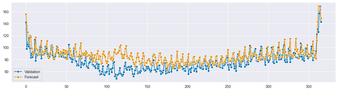
plot_forecasts(val_targets_xgboost_tuned, forecast_xgboost_tuned, title="XGBoost Tuned Forecasts");

Code

print(f"MAPE for Earlier XGBoost model is: {mean_absolute_percentage_error(test_targets_xgboost, forecast_xgboost)}")
print(f"MAPE for Tuned XGBoost model is: {mean_absolute_percentage_error(val_targets_xgboost_tuned, forecast_xgboost_tuned)}\n")

print(f"R2 Score for Earlier XGBoost model is: {r2_score(test_targets_xgboost, forecast_xgboost)}")
print(f"R2 Score for Tuned XGBoost model is: {r2_score(val_targets_xgboost_tuned, forecast_xgboost_tuned)}\n")

print(f"Total Cost for Tuned XGBoost model is: €{xgboost_total_cost:,.2f}")

MAPE for Earlier XGBoost model is: 0.09307335208975362
MAPE for Tuned XGBoost model is: 0.1657821900657774

R2 Score for Earlier XGBoost model is: 0.6931165642563528
R2 Score for Tuned XGBoost model is: 0.10051546999689664

Total Cost for Tuned XGBoost model is: €60,058.00

Tuning for XGBoost model loses some accuracy due to the difference between lagged value features. Earlier model was using real targets as lagged value, while this tuned and correct model uses its own forecasts as lagged values. We’ll create and tune deep learning models on

Part 2 ->